About the Neutronics Scoping Tool

Much can be known about a nuclear reactor from relatively simple analysis tools. We made the Neutronics Scoping Tool to help build an intuition for the core performance of different reactor types, fuels, and enrichments. If you haven’t tried it out yet, click that link, play around with it, and then come back for more info. You can also watch me play with it in this screenshare.

Using it, you can quickly:

• Estimate how much fuel is needed to go critical at a certain reactor size
• Estimate how long a reactor can stay critical at various power ratings
• Visualize core size and shielding at different sizes in interactive 3D with person for scale
• Understand how down-rated or up-rated a given power level is for a given core size (e.g. compared to ‘typical’ reactors of a type)
• See the fuel cost and Levelized Cost of Electricity from nuclear fuel
• Estimate how much control is required
• Estimate average discharge burnup for a given core

So if someone says they have a SFR that fits in a Volkswagen and can run for 10 years, you can use this tool to roughly understand their core characteristics. This is intended to be helpful for the interested public, engineers, and investors navigating the nuclear space.

At the moment, only a few common reactor types are supported: Pressurized Water Reactors (PWRs), High Temperature Gas-cooled Reactors (HTGRs), and Sodium-cooled Fast Reactors (SFRs). We will add more as we do more unit cell calcs.

How it works

The scoping tool consists of a core model with inputs, and the resulting reactivity vs. time curve. The core model is defined by the following user-selectable inputs:

• Reactor type
• Core radius
• Core height
• Fuel enrichment
• Power rating (%)
• Cycle length override (optional and not recommended)

Each supported reactor type is tied to an assumed fuel pin-cell design, which includes:

• Fuel material and dimensions
• Clad material and dimensions
• Coolant material
• Moderator material
• Typical power density

Without any real nuclear reactor physics, the inputs alone set some key parameters, like:

• Fuel mass (if you input the core dimensions, enrichments, and unit cell, you can compute mass)
• Fuel cost (derived from mass and enrichment)
• Core heavy metal density (just fuel mass divided by core volume)
• Shielding required (basically wrapping the core volume in a blanket of shielding)

Computing the reactivity vs. time curve is the hard part. Doing this requires neutronics calculations with depletion. I’ve gone ahead and built unit cell inputs and run them for you. The unit cell calcs provide:

• Reactivity vs. time in an infinite medium
• Migration area

I used the open-source reactor physics codes DRAGON and OpenMC using ENDF/B-VII.1 cross section input.

DRAGON is a self-proclaimed legacy code developed at École Polytechnique de Montréal for decades. It’s a true expert code that can model almost all reactor types with extreme computational efficiency. It’s somewhat hard to learn and has lots of modeling and approximation settings that you can accidentally abuse if you’re not careful.

OpenMC is a powerful Monte Carlo neutronics code maintained originally at MIT and now Argonne National Lab. It can model any geometry and has very few approximations or knobs, making it much easier to use and believe. Its disadvantage is that it is computationally expensive (less of an issue these days since reactor development teams often have supercomputers and/or clouds at their fingertips).

I ran both of them as a Quality Assurance step: OpenMC gives me what I’m considering a reference solution but runs for some hours, and DRAGON gives me much more information faster. So all the unit cell results in the scoping tool are coming from DRAGON, but I spot-checked some of the DRAGON cases with longer-running OpenMC cases to make sure I was using DRAGON correctly.

I ran infinite (reflective boundary) DRAGON cases at 10 different enrichments between natural and 20% with depletion at typical power densities for each reactor type. The data was loaded into the web applet, which interpolates linearly between the 10 enrichments to find the curve that matches whichever enrichment the user selects.

A leakage approximation is applied based on the core dimensions selected. The k-infinite curves are converted to k-effective curves through the following expression:

\[\text{k}_{eff} = \frac{\text{k}_{\infty}}{1 + M^2 B^2}\]

where:

• \(k_{eff}\) is the reactivity with leakage
• \(k_{\infty}\) is the reactivity in an infinite array
• \(M^2\) is the transport-corrected migration area, related to the distance a neutron travels from birth to absorption
• \(B^2\) is the geometric buckling in a bare cylinder, which (as anyone familiar with Bessel functions knows) is related to the core height H and radius R as: \((\frac{\pi}{H})^2 +(\frac{2.405}{R})^2\)

H and R are user inputs, and we get \(M^2\) and \(k_{\infty}\) from the DRAGON interpolations. Thus, we have a full reactivity vs. time curve!

Note that this approximation doesn’t work well for very small cores, which is why the tool becomes extra wrong then cores get too small. That’s why it’s limited in how small you can make it on the sliders.

For the power rating, a reactor making 100 watts for 100 days is neutronically identical to one making 1 watt for 10,000 days or, equivalently, 10,000 watts for 1 day. Thus, as the user slides the power rating from 1% to 200%, the tool simply rescales the time axis.

With each update, the reactivity curve is interpolated/extrapolated to \(k_{eff} = 1.0\) to estimate the cycle length. After your reactor goes below 1.0, it needs to be reloaded.

The fuel LCOE is computed using the same unit cost assumptions in the SWU calculator. Your cycle is repeated for approximately 60 years of reactor life. The NPV of the fuel costs is divided by the NPV of the electricity generated, both discounted at 8%.

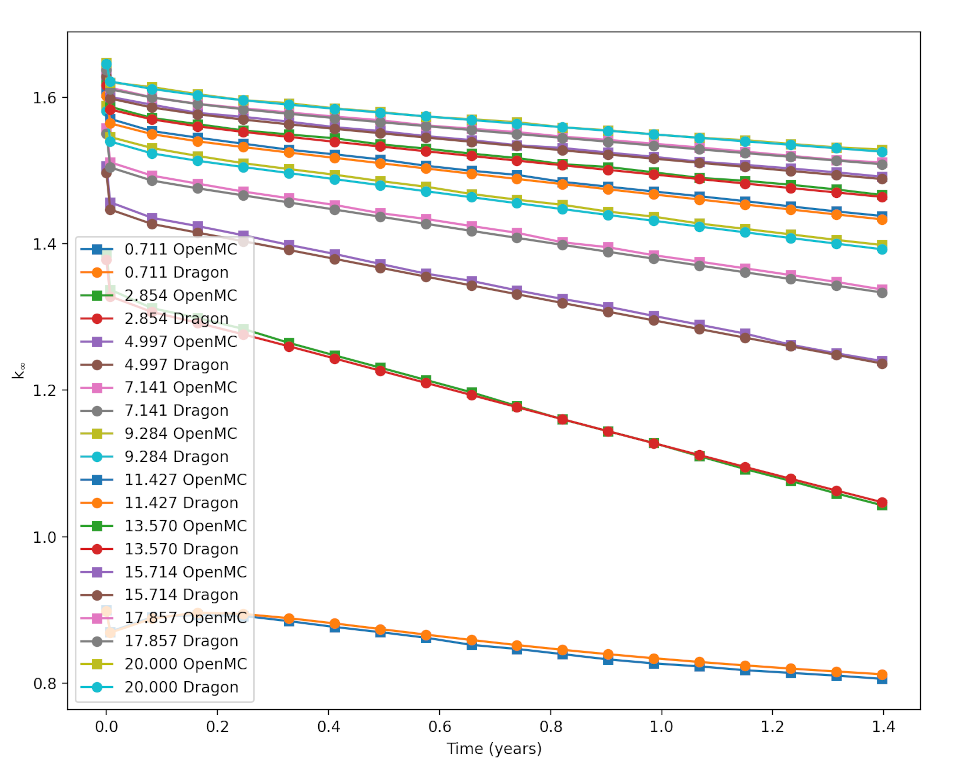
LWR unit cell

The LWR unit cell here is literally the one defined in the example problem that comes with OpenMC. It is depleted with a typical LWR power density.

The infinite case benchmarking looked quite good. I hammered the OpenMC cases for this, at least given my limited personal computational power. I’d say DRAGON is doing just fine. The OpenMC cases took about 7 hours on my PC all in, and the DRAGON cases took about 2 minutes.

The leakage approximation was benchmarked against finite-geometry calculations in OpenMC (one big fininte cylinder of unit cells). At 30 x 15 cm, the scoping tool was overestimating keff by 15,000 pcm! Anything bigger than radius 30, height 60 had errors between 100 and 6,000 pcm. The overestimation will generally be counteracted by reflectors so I figure it’s still ok for basic scoping. But don’t get too excited about high keffs for tiny cores.

HTGR unit cell

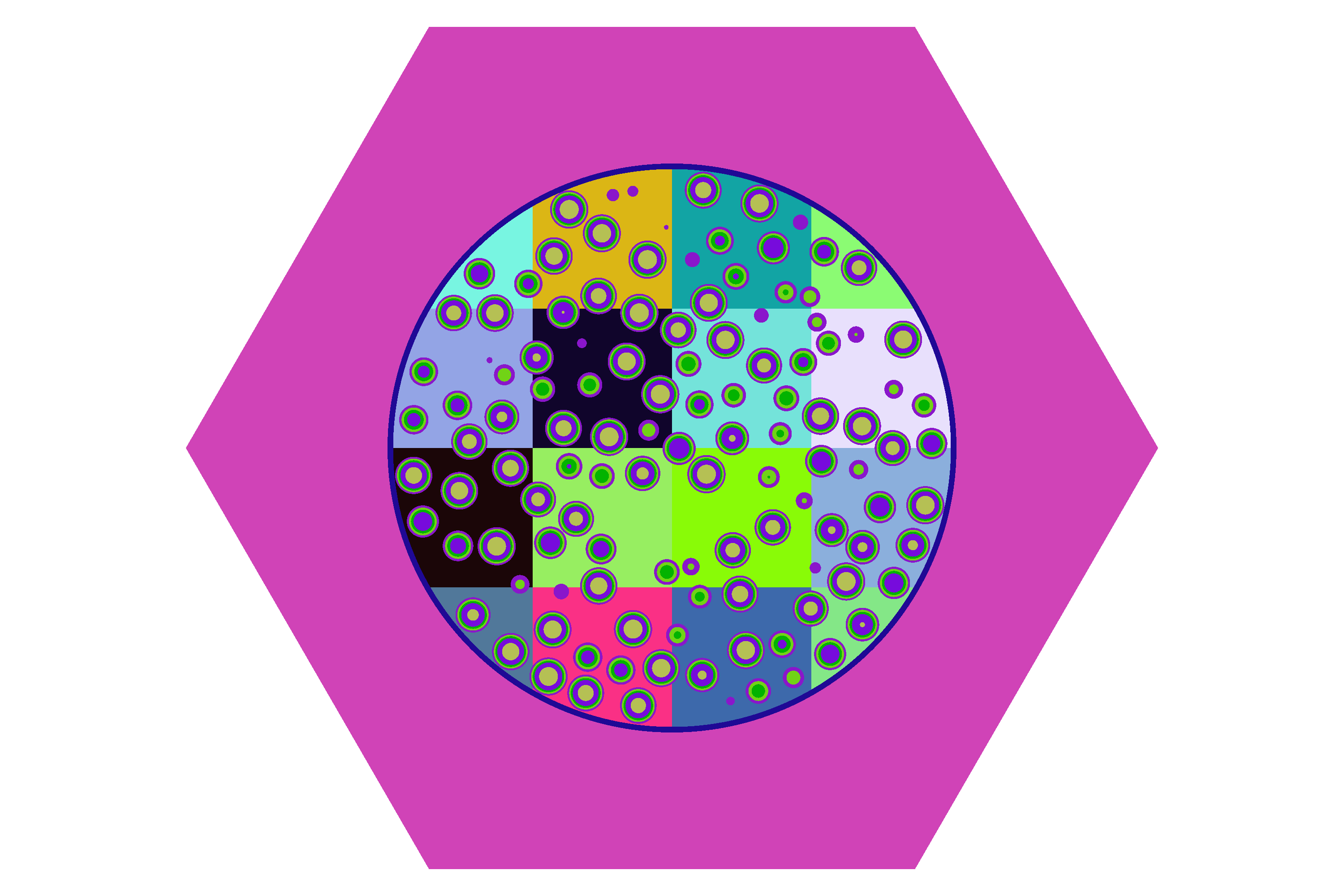
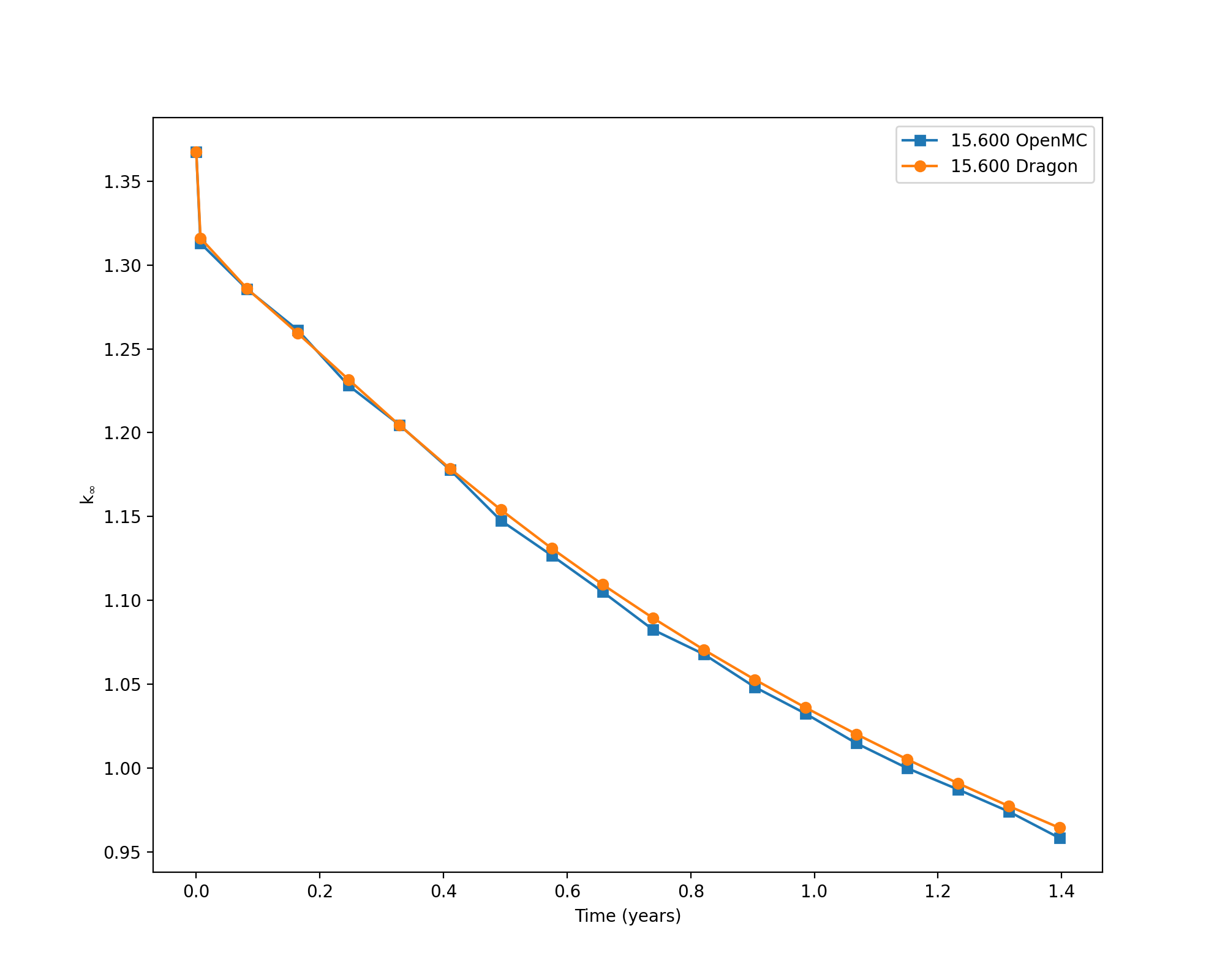
The HTGR unit cell is based on a MHTGR benchmark from (Strydom & Bostelmann, 2015). This benchmark was evaluated in DRAGON and MCNP in (Skerjanc, 2017) and therefore gave me a baseline by which I could compare both my DRAGON and OpenMC cases. Modeling TRISO fuel is slightly more complicated because of the double heterogeneity, where we have the tiny TRISO particles at one level and then an array of compacts in tubes as another level. This is a prismatic model (as opposed to pebble bed). A typical HTGR power density is applied for depletion.

I ran an OpenMC depletion case with very few neutrons this time so some stochastic noise is evident.

SFR unit cell

The SFR unit cell is a 0-D homogenized inner-fuel region from the 1.0 Conversion Ratio metallic core published in ANL-AFCI-177 (Hoffman et al., 2008). Input files are already available online for that core as well as open-source code to run DRAGON for these. The core was run at a typical SFR power density of 354 W/cc.

Tips and Observations

• You might think you want to down-rate your reactor to make it stay critical longer. This is a cool selling point and makes passive decay heat removal easier. But keep an eye on the fuel LCOE. When you downrate, your fuel LCOE skyrockets. You may be pressured by customers to increase power for this reason.

• Keep an eye on your fuel burnup. Just because you pack in enough reactivity to stay at power for a long time, if you go beyond the burnup that your fuel form can handle, it will fail on you and release fission products well before you run out of reactivity. The peak/average shown is easy to reduce via fuel shuffling and burnable poisons, so pay most attention to the average.

• Reactivity swing can also be a killer. You can only compensate for so much change in reactivity with a control system. And if you put in extremely strong absorbers, remember that you have to handle the accident where the highest worth one ejects or melts or otherwise disappears. You can reduce reactivity swing by breaking a cycle up into smaller cycles and performing fuel management, but then you’ll have more downtime and need more automated fuel handling equipment.

• TRISO fuel has about 5% the fuel density as regular UO₂. The kernels themselves are 12% fuel by volume, and they’re packed into compacts or pebbles at about 35% packing fraction, so… you do the math. Having less fuel means neutrons have more trouble finding the next uranium atom, and are more likely to leak out the sides or top. You can reflect them back in, but only to a degree. Neutrons aren’t too apt to turn around. That said, the physical robustness and high-temperature capability of TRISO fuel still brings a lot of appeal.

• Water is a hell of a moderator. It’s hard to beat the fact that hydrogen can slow down neutrons to thermal speeds in one shot. You’ll see that the migration length in water is like 4 cm, vs more than 20 cm in the HTGR cell. This means that you need a lot more moderator volume per power in a HTGR than a LWR. The astounding compactness of LWRs is why Rickover chose them over the Daniels Pile HTGR for Nautilus.

• Some metrics sort of break down for breeders. When you run the SFR with a medium enrichment at or below 8-12%, you’ll see that \(k_{eff}\) goes up over time due to breeding plutonium. Given this, the extrapolated cycle length may not make a lot of sense, and you might need to take control of the cycle length (by unchecking the auto checkbox). As with the rest of the tool, use with care.

Getting the actual answer

To do real design work on a nuclear reactor, you need to model the full core, including reflectors, shields, control, and burnable poisons. The control rods need to be moving to their critical positions at all timesteps and the control material should be depleting. This perturbs the neutrons in space and will impact your overall performance. Reflectors and fuel management will even out radial burnup peaking. You should be optimizing the lattice for your specific case, computing reactivity coefficients and shutdown margins, estimating phase and gain margins of stability, and running transient analysis for all your design-basis accidents and some beyond design basis ones to ensure your design satisfies its constraints in all bounding accident scenarios. You need detailed coolant flow models based on experimental data to know flow rates, pressure drops, and hot channel factors. You need fuel performance models to know if the fuel can survive limiting transients as well. Ah, the joys of nuclear simulations!

Once you’re done scoping, plan to write up a conceptual design. Here’s an example (ORNL Staff, 1962) of about the right amount of detail for a nuclear conceptual design.

Feedback and suggestions

If you have ideas or bug reports on how to improve the scoping tool, hit me up!

References

1. Strydom, G., & Bostelmann, F. (2015). IAEA Coordinated Research Project on HTGR Reactor Physics, Thermal-hydraulics and Depletion Uncertainty Analysis (INL/EXT-15-34868; Number INL/EXT-15-34868). Idaho National Lab. (INL), Idaho Falls, ID (United States). https://doi.org/10.2172/1244621
2. Skerjanc, W. F. (2017). HELIOS vs. DRAGON – Code-to-Code Comparison for High Temperature Gas Reactors (INL/MIS-17-41227-Rev000; Number INL/MIS-17-41227-Rev000). Idaho National Lab. (INL), Idaho Falls, ID (United States). https://www.osti.gov/biblio/1556111
3. Hoffman, E. A., Yang, W. S., & Hill, R. N. (2008). Preliminary Core Design Studies for the Advanced Burner Reactor over a Wide Range of Conversion Ratios. (ANL-AFCI-177; Number ANL-AFCI-177). Argonne National Lab. (ANL), Argonne, IL (United States). https://doi.org/10.2172/973480
4. ORNL Staff. (1962). CONCEPTUAL DESIGN OF THE PEBBLE BED REACTOR EXPERIMENT (Report ORNL- TM- 201; Number ORNL- TM- 201). ORNL. https://doi.org/10.2172/4829552

See Also

• Neutronics Scoping Tool
• Screenshare demo of the scoping tool
• Our Fuel Cost/SWU Calculator