This page derives the basic equation of radioactive decay. This equation allows us to figure out how many radioactive atoms are left after any amount of time. There are many general forms of the equation that deal with chains of nuclides, but here we only worry about the basics. WARNING: there is a little bit of calculus involved.

Try out our Interactive half-life calculator!

Number of atoms at any given time

We start by noting that the speed of radioactive decays occurring in a sample is proportional to the number of radioactive atoms in the sample. This isn’t hard to believe. If you had 10 jumping beans and saw one jump every second, you’d expect to see about 10 jumps per second if you had 100. Mathematically, we represent this as $$-\frac{dN}{dt}=N\lambda$$ where \(\frac{dN}{dt}\) is the number of decays per second the batch of atoms is undergoing, \(N\) is the current number of radioactive atoms, and \(\lambda\) is a constant (called the decay constant) which is characteristic of any particular radioactive atom representing the likelihood that any individual atom will decay at any given time. Atoms that decay faster have larger decay constants, and so on.

Now that we know the rate at which our sample is decaying, we can integrate this rate to figure out the total number of atoms that have decayed at any given time. Unfortunately we can’t just multiply by time because the decay rate is changing as the number of atoms changes. So we’re forced to use calculus. Here we go, step-by-step: $$ \begin{aligned} \frac{dN}{N} &= -\lambda dt && \text{Rearrange to get } N \text{ on one side}\\ \int_{N_0}^{N} \frac{dN}{N} &= -\lambda \int_{t=0}^t dt && \text{Integrate over the interval of interest}\\ \text{ln}\left({N}\right)-\text{ln}\left(N_0\right) &= -\lambda t && \text{Evaluate the integrals}\\ \text{ln}\left(\frac{N}{N_0}\right) &= -\lambda t && \text{Use log rules to combine the left-hand side}\\ \frac{N}{N_0} &= e^{-\lambda t} && \text{Take } e \text{ to the power of both sides}\\ N &= N_0 e^{-\lambda t} &&\text{Multiply both sides by } N_0\\ \end{aligned}$$ Note: \(N_0\) is the number of nuclides at time \(t=0\).

Relating the half-life to the decay constant

Excellent. The final equation there is the well-known radioactive decay equation. But what should we use for \(\lambda\)? You may have heard of the concept of half-life, or \(\tau_{1/2}\). It’s the time it takes for a batch of radioactive atoms to decay away, i.e. the lifetime of half of the atoms. We can relate \(\tau_{1/2}\) to \(\lambda\) easily using the formula derived above. We just say we start with \(N_0=100\) atoms and calculate the \(t\) it takes for this to drop to \(N=50\). $$\begin{align} 50 &= 100 e^{-\lambda \tau_{1/2}} &&\text{Plug in desired values, and } t=\tau_{1/2}\\ \left(\frac{50}{100}\right) &= e^{-\lambda \tau_{1/2}} \\ \left(\frac{100}{50}\right) &= e^{\lambda \tau_{1/2}} && \text{Take reciprocal of both sides}\\ \text{ln}(2) &= \lambda \tau_{1/2} &&\text{Take the ln of both sides}\\ \lambda &= \frac{\text{ln}(2) }{\tau_{1/2}} && \text{Obtain expression for } \lambda \text{ vs. half-life}\\ \end{align}$$

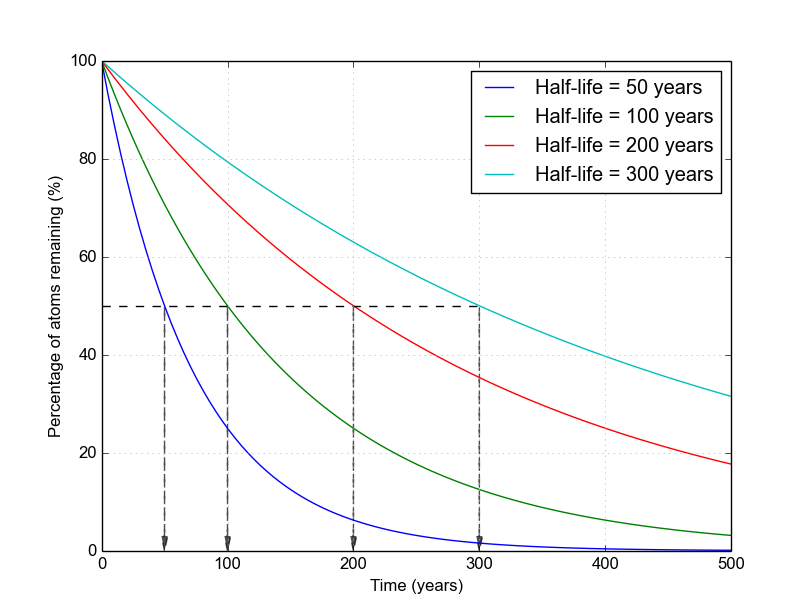
As a visual example of how nuclide populations change with different half-lives, take a look at this figure below. All nuclides start out with 100% of their atoms. The blue curve represents a nuclide that has a 50-year half-life. As you can see, it reaches 50% at exactly 50 years. Compare this with the green curve, which represents a nuclide with a 100-year half-life. It crosses 50% exactly at 100 years. And so on.

Figure 1. Decays of several example nuclides with different half-lives from 50 to 300 years. The Python code to generate this image is available here.

Population of daughter nuclides

It’s often useful to know the population of a decay product of a radioactive decay (also known as a daughter nuclide). These may be useful for radiogenic dating of objects (like the Earth), understanding nuclear waste behavior, etc. Let the number of daughter nuclides at \(t=0\) be \(D_0\). Then, $$ \begin{align} D &= D_0 + N_0 - N &&\text{Because } N_0 - N \text{ parent nuclides decayed}\\ &= D_0 + N_0 -N_0 e^{-\lambda t} &&\text{Plugging in the decay equation}\\ &= D_0 + N_0\left(1-e^{-\lambda t} \right) &&\text{Final form based on } N_0\\ &\text{or, if you want a formula based}\\ &\text{on current parent population, } N\\ &= D_0 + Ne^{\lambda t}\left(1-e^{-\lambda t} \right)&& \\ &= D_0 + N \left(e^{\lambda t}-1 \right)&& \text{Alternate form based on current } N\\ \end{align}$$

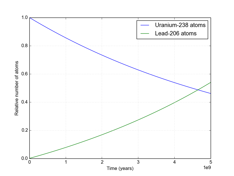
An example of Uranium-238 (with a 4.47 billion year half-life) decaying into Lead-206 is shown in Figure 2, where we assume \(D_0 = 0\). Notice that the sum of these two curves is always 1.0.

Figure 2. The decay of Uranium-238 eventually leads to Lead-206. There are many steps along the way, but they all have very short half-lives compared to that of U-238 so they can be ignored on these long (geologic) time scales. Find details of the decay chains here.

---

See Also

1. The Radioactive Decay [Wikipedia] page has a much more detailed and thorough description of radioactive decay, including situations with more complex decay chains.
2. KAERI Chart of the Nuclides has lots of half-lives you can look up

References

1. Dickin, A.P, 2005. "Radiogenic Isotope Geology." United Kingdom: University Press, Cambridge.